EMA: A Quiet Hyperparameter That Moves Diffusion Leaderboards
Diffusion transformers are increasingly compared by convergence speed: who can reach a target FID in the fewest training epochs. But before changing the model architecture, loss, or input space, one quiet hyperparameter can already move the number: EMA decay. In the figure below, we take the same RAE-DiT1 training run at 80 epochs and change only the EMA decay. The gFID moves from 4.14 to 3.21. This is large enough that two papers could appear to differ in method quality when they are partly differing in EMA protocol.
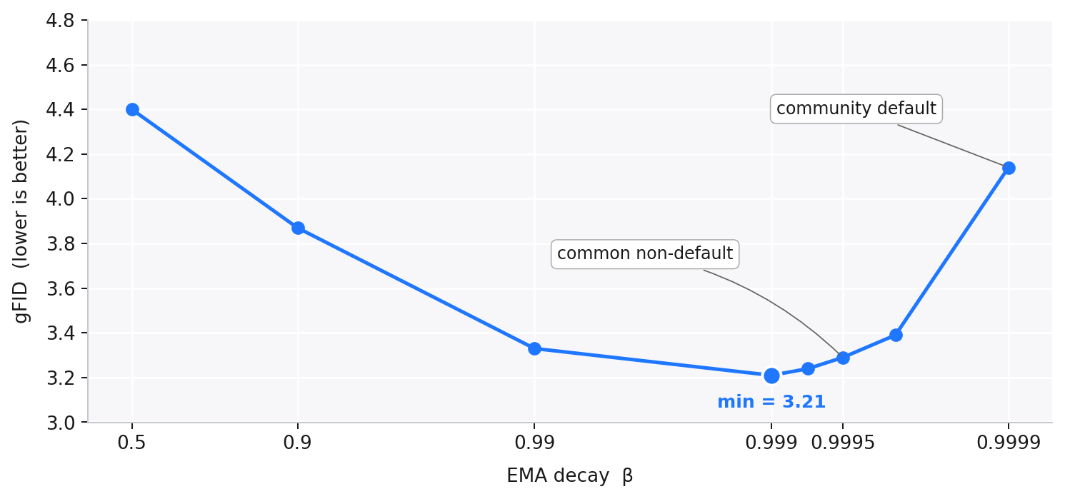
This plot is the instability we want to make visible. EMA decay is often treated as a fixed detail of the training recipe rather than a hyperparameter to study. But the plot above shows the key point: common EMA choices are not interchangeable. Later, the reporting table shows how often these choices are inherited from existing codebases or left implicit in recent diffusion papers.
The rest of the post asks two questions. First, when diffusion models are evaluated before full convergence, how much can EMA decay change the comparison? Second, what does EMA decay change inside the learned distribution? We study three settings: representation-space diffusion (RAE1), pixel-space diffusion (JiT2), and latent-space diffusion (SiT3).
Why Did EMA Become the Default?
Exponential moving average (EMA) keeps a slowly updated copy of the model weights alongside the training weights. At every optimizer step t, the EMA weights θ′ are updated as
$$\theta'_t \;=\; \beta \, \theta'_{t-1} \;+\; (1 - \beta)\, \theta_t\,,$$
where β is the EMA decay. At evaluation time, samples are drawn from θ′ instead of θ: the running average, not the latest optimizer step. That sounds like harmless smoothing, and historically that is exactly why EMA became popular.
The NCSNv2 example below shows the original motivation. EMA was introduced to diffusion models as a fix for a very visible failure mode: color shift4. Without EMA, samples near the end of training drifted in color statistics, even when the score loss kept decreasing. The EMA checkpoint smoothed the trajectory and brought the sample statistics back in line.
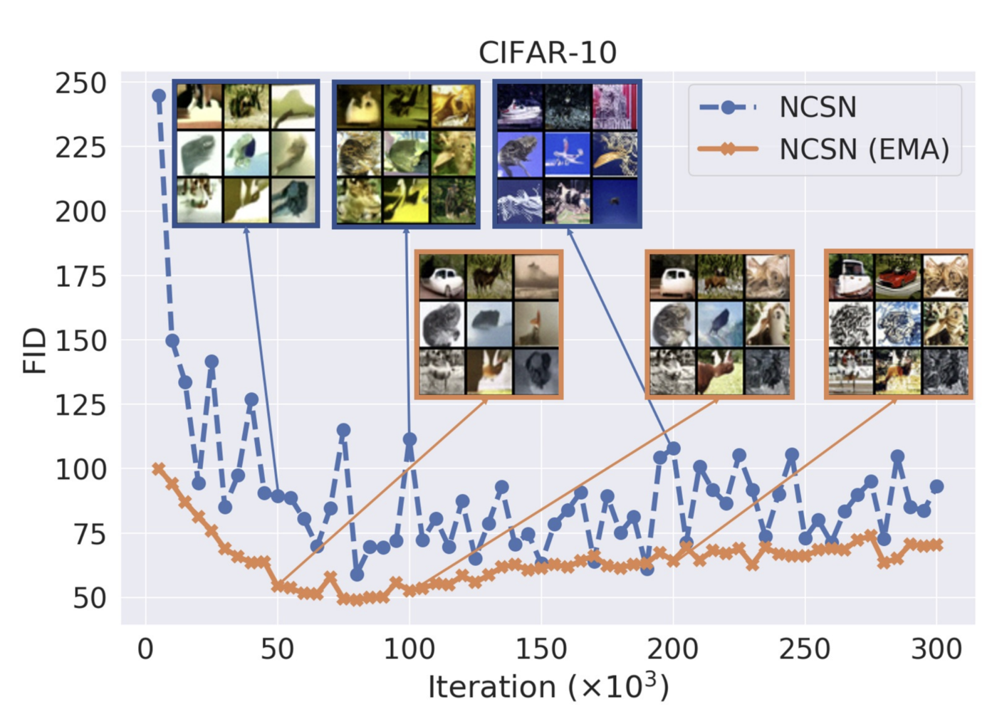
This figure explains why EMA became a near-universal default: the fix is obvious, visual, empirically useful, and almost free. In our sweeps, EMA-smoothed checkpoints also beat the raw checkpoint across pixel-, latent-, and representation-space diffusion. So the question is not whether EMA helps. It does. The question is whether the decay rate can be left on autopilot.
That distinction matters most away from convergence. If the goal is a final, near-converged FID, the exact averaging window may look less central: late in training, the weights move more slowly, and different EMA averages can become similar. But at 40 epochs, 80 epochs, or any target-FID speed benchmark, the trajectory is still moving quickly. Different EMA decays can then correspond to very different evaluated checkpoints.
Short-Schedule FID Makes EMA Visible
That lag becomes a measurement problem because diffusion papers usually report the EMA checkpoint. An FID number is therefore not determined only by the method, optimizer, and training budget; it also depends on the EMA decay used to build the checkpoint. The reporting landscape below shows why this is easy to miss.
| Method | Parent Codebase | Reported EMA Decay | Epoch 40 | Epoch 80 | EPFID@3 | Open Sourced? |
|---|---|---|---|---|---|---|
| DiT5 | - | 0.9999 | 39 | 16 | >800 | Yes |
| SiT3 | DiT5 | 0.9999 | 34 | 15 | >800 | Yes |
| JiT2 | DiT5 | 0.9999 | - | 42.9 | >800 | Yes |
| REPA6 | DiT5, SiT3 | 0.9999 | 10.5 | 7.9 | >800 | Yes |
| RAE1 | LightningDiT7 | 0.9995 | 6.7 | 4.3 | 200 | Yes |
| RJF8 | RAE1 | 0.9995 | - | 3.6 | 80~85 | No |
| FAE9 | RAE1 | - | 2.8 | 2.1 | 35~40 | No |
| RAEv210 | RAE1 | 0.9995 | 2.8 | 2.3 | <20 | Yes |
| PAE11 | RAE1 | 0.9999 | 5.8 | 1.9 | 45~50 | Yes |
The table matters because recent comparisons increasingly live at intermediate checkpoints. Final FID still appears, but many papers now emphasize fixed-budget FID at 40 or 80 epochs, or the number of epochs needed to hit a target FID. RAEv210 makes one piece of this shift explicit:
RAEv2 on Training-Convergence Evaluation10"Incremental improvements in absolute gFID values might provide limited signal for practical applications. Inspired by recent speedrun in language domain, we also report training convergence using EPFID@k (epochs to reach unguided gFID ≤ k)."
RAEv2 therefore reports EPFID@k: the number of epochs needed to reach unguided gFID ≤ k. This is a useful direction because it asks how much training a method needs to become good enough, not just where it lands after a long run. But the curve being thresholded is usually the EMA-smoothed curve. If changing β moves that curve, it can also move the apparent convergence time.
The figure below shows this within a single RAE-DiT1 run. All curves come from the same optimizer trajectory; only the EMA decay changes. At target k = 4, that choice changes the apparent convergence time from 32 epochs to beyond 80 epochs.
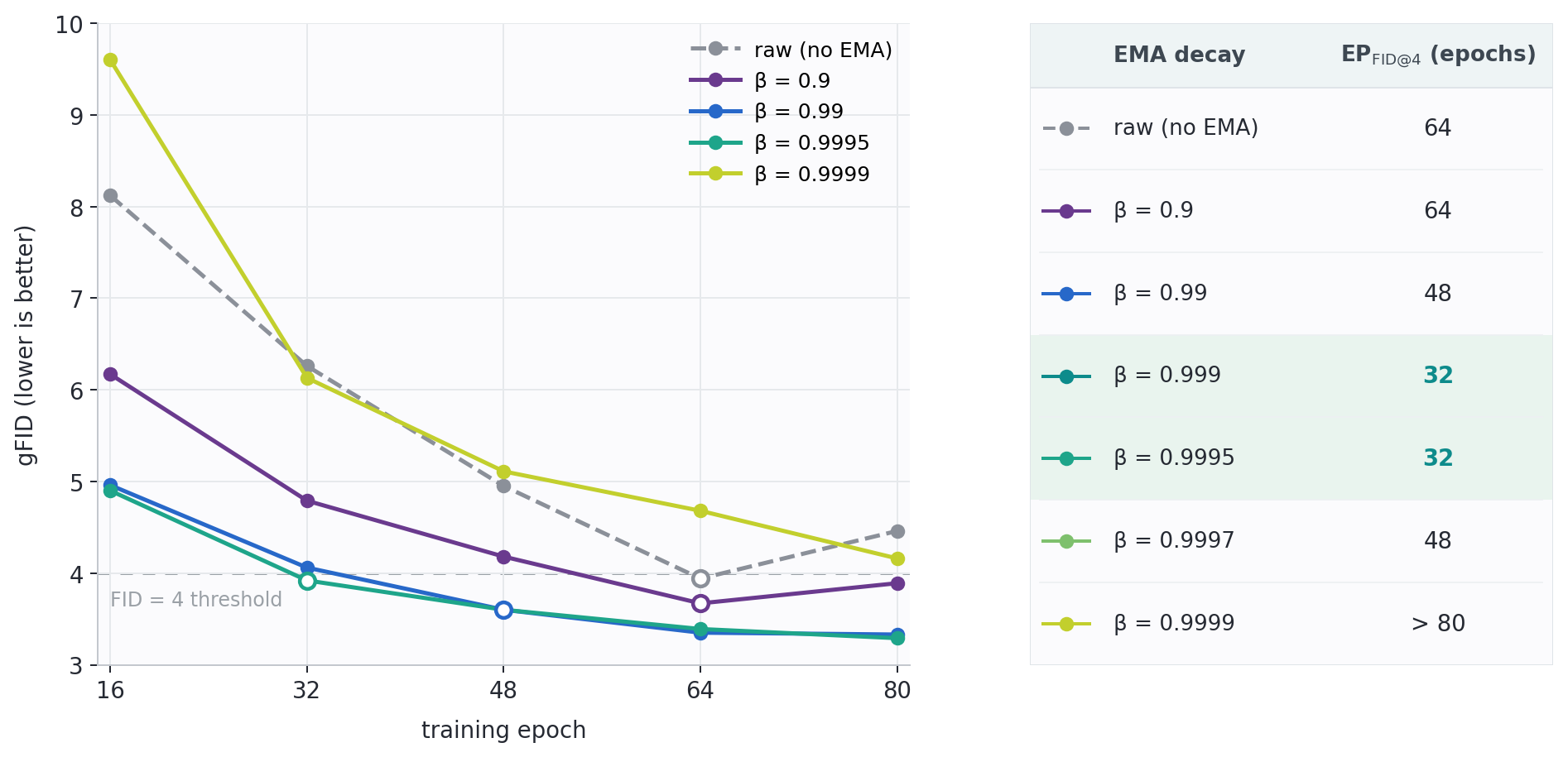
Read together, these results show why fixed-budget FID and EPFID@k need a matched EMA protocol. If two methods use different decays, the reported gap can reflect both the proposed method and the EMA checkpoint used to evaluate it.
That motivates the controlled sweeps in the next section: if EMA decay can change both the number and the crossing time, what exactly is it changing in the learned distribution?
EMA Trades Precision for Recall
We showed that EMA decay can change the reported FID. Here we ask what changes inside the learned distribution. The answer is not simply "better" or "worse": EMA decay moves the model along a precision-recall trade-off. Larger decays tend to sharpen samples and raise precision, but they also reduce coverage and lower recall.
The intuition is that EMA rewards what is stable across time. Common patterns survive the averaging window and become cleaner; rare or fragile modes are more easily averaged away. So the model looks more precise, but it covers less of the distribution.
To isolate this effect, we sweep EMA decay for three diffusion models spanning common input spaces: JiT2 in pixel space, SiT3 in latent space, and RAE1 in representation space. Each sweep also includes the raw online checkpoint.
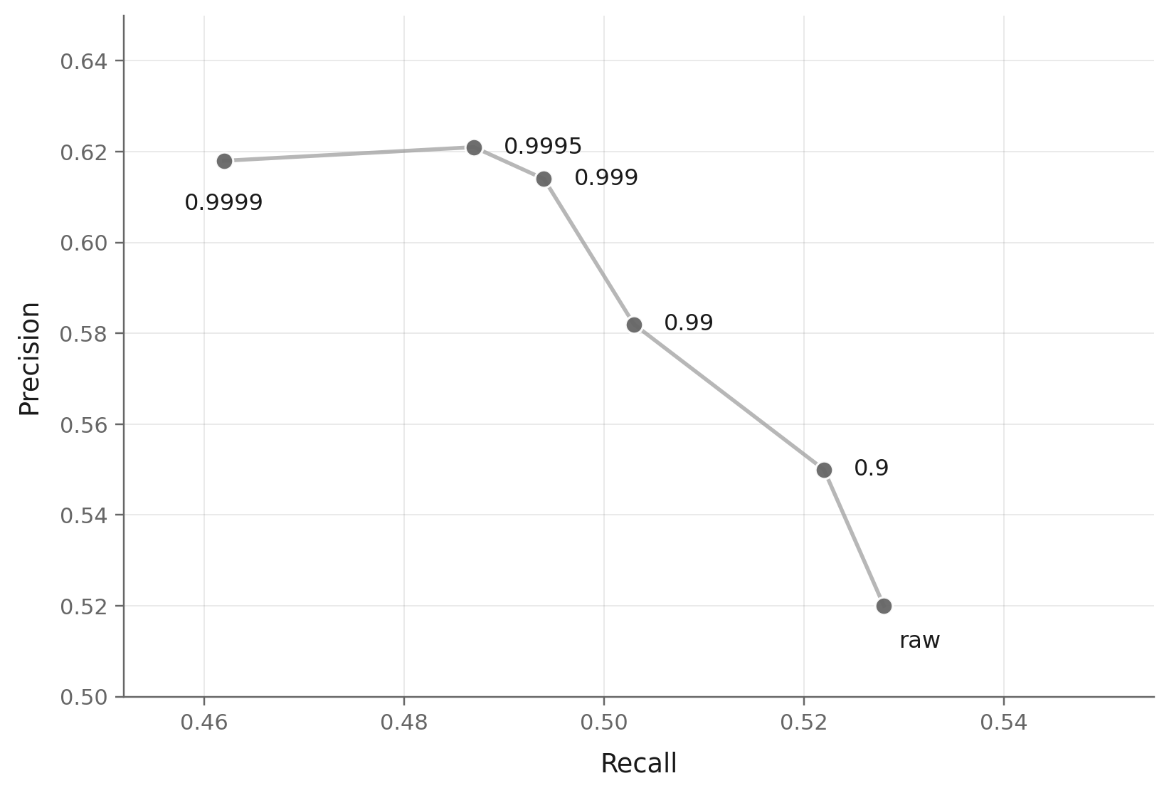
The RAE sweep makes the mechanism visible. Every point below comes from the same online training trajectory; only the EMA decay used to form the checkpoint changes.
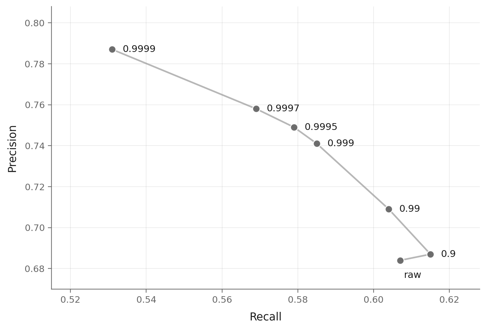
This is the key mechanism. Moving from raw to β = 0.9999, precision rises from 0.68 to 0.79, while recall falls from 0.61 to 0.53. No single decay wins on both axes. EMA does not only smooth optimization noise; it dials the model between fidelity and coverage.
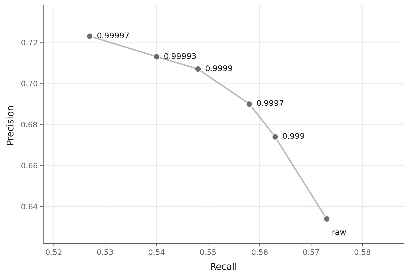
The same pattern holds in pixel and latent spaces. JiT and SiT show the same broad direction: as decay grows, precision tends to improve and recall tends to shrink. The exact curve shape differs by model, but the effect is not specific to RAE.
This also explains why there is no universally best decay. FID is sensitive to both fidelity and coverage, so it tends to reward a compromise point on the precision-recall curve. Precision-like metrics can prefer larger decays. Recall prefers smaller decays. Once EMA decay moves the precision-recall ratio, different metrics naturally select different decays.
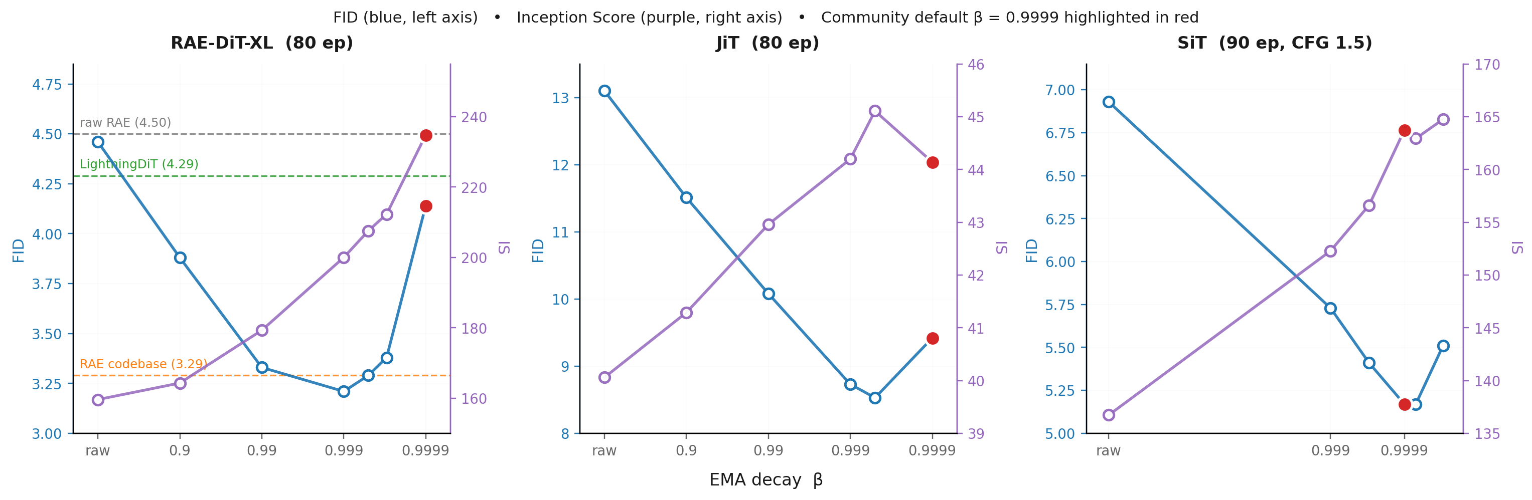
RAE is the cleanest example: FID is best at β = 0.999, while Inception Score keeps improving toward larger decays. JiT is different: β = 0.9995 is best on both FID and IS in this sweep. SiT is milder: FID is nearly flat around the high-decay region, while IS keeps rising. The common lesson is not that one decay is always right. The lesson is that EMA decay changes the distributional trade-off, so the metric decides which decay rate serves best.
Soft Collapse in a 2D Toy
The ImageNet sweeps show the metric-level effect: larger EMA decay raises precision and reduces recall. The toy example below shows the same effect at the sample level. We use a 2D distribution from AutoGuidance14: a tree with dense, popular branches and sparse tail branches. If recall drops, those tail branches should be the first places to disappear.
We train one small MLP score model, then compare the raw model with EMA versions at
0.99 / 0.997 / 0.998 / 0.999. The first figure is the sweep overview: read it left to
right as EMA decay increases.
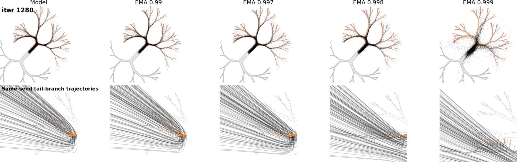
The most useful comparison is not the catastrophic 0.999 case. It is the softer
0.998 case: samples still look plausible, but coverage has already changed.
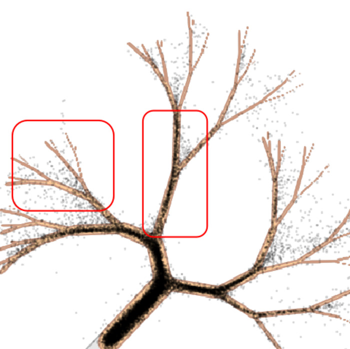
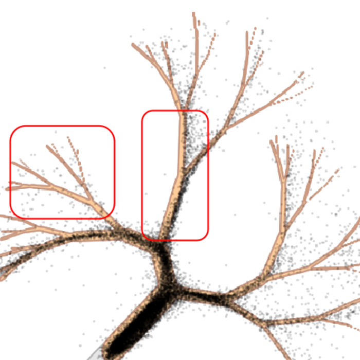
This is not a hard collapse to a single mode. It is softer: EMA over-concentrates the model on high-density regions. That explains the precision-recall trade-off from the previous section. Samples can look cleaner because they hug typical patterns more tightly, while rare configurations quietly lose coverage.
Closing Remarks
EMA is easy to trust because it is genuinely useful. It stabilizes sampling, improves raw checkpoints, and has become part of the default diffusion training recipe. But the decay rate is not just an implementation detail: it changes which checkpoint we evaluate and where the model sits on the precision-recall curve.
Our practical recommendation is simple: report the EMA decay, and treat it as part of the evaluation protocol. For short-schedule comparisons, fixed-budget FID at 40 or 80 epochs, or EPFID@k, matched EMA settings matter. When possible, sweep EMA under a shared protocol; at minimum, an early FID number should come with the EMA decay that produced it.
Several questions remain open. Can the precision-recall trade-off be characterized directly from how EMA reshapes the score function? Does the optimal β drift predictably with training horizon, model size, or guidance scale? If so, adaptive EMA, scheduled EMA, or post-hoc EMA methods such as EDM215 could make matched comparisons routine rather than expensive. Until then, the cheapest safeguard is also the simplest: whenever you report a short-schedule number, report the EMA decay that produced it.
References
- Zheng, Ma, Tong, & Xie. Diffusion Transformers with Representation Autoencoders. ICLR, 2026. arXiv:2510.11690. ↩︎
- Li & He. Back to Basics: Let Denoising Generative Models Denoise. CVPR 2026. arXiv:2511.13720. ↩︎
- Ma, Goldstein, Albergo, Boffi, Vanden-Eijnden, & Xie. SiT: Exploring Flow and Diffusion-based Generative Models with Scalable Interpolant Transformers. ECCV 2024. arXiv:2401.08740. ↩︎
- Song & Ermon. Improved Techniques for Training Score-Based Generative Models. NeurIPS 2020. arXiv:2006.09011. ↩︎
- Peebles & Xie. Scalable Diffusion Models with Transformers. ICCV 2023. arXiv:2212.09748. ↩︎
- Yu, Kwak, Jang, Jeong, Huang, Shin, & Xie. Representation Alignment for Generation: Training Diffusion Transformers is Easier than You Think. ICLR 2025. arXiv:2410.06940. ↩︎
- Yao, Yang, & Wang. Reconstruction vs. Generation: Taming Optimization Dilemma in Latent Diffusion Models. CVPR 2025. arXiv:2501.01423. ↩︎
- Kumar & Patel. Learning on the Manifold: Unlocking Standard Diffusion Transformers with Representation Encoders. arXiv preprint, 2026. arXiv:2602.10099. ↩︎
- Gao, Chen, Chen, & Gu. One Layer Is Enough: Adapting Pretrained Visual Encoders for Image Generation. arXiv preprint, 2025. arXiv:2512.07829. ↩︎
- Singh, Zheng, Wu, Zhang, Shechtman, & Xie. Improved Baselines with Representation Autoencoders. arXiv preprint, 2026. arXiv:2605.18324. ↩︎
- Yue, Hu, Chen, Zhang, Pan, Liu, Wang, Lan, Zhu, Zheng, & Wang. What Matters for Diffusion-Friendly Latent Manifold? Prior-Aligned Autoencoders for Latent Diffusion. arXiv preprint, 2026. arXiv:2605.07915. ↩︎
- Kynkäänniemi, Karras, Laine, Lehtinen, & Aila. Improved Precision and Recall Metric for Assessing Generative Models. NeurIPS 2019. arXiv:1904.06991. ↩︎
- Salimans, Goodfellow, Zaremba, Cheung, Radford, & Chen. Improved Techniques for Training GANs. NeurIPS 2016. arXiv:1606.03498. ↩︎
- Karras, Aittala, Kynkäänniemi, Lehtinen, Aila, & Laine. Guiding a Diffusion Model with a Bad Version of Itself. NeurIPS 2024. arXiv:2406.02507. ↩︎
- Karras, Aittala, Lehtinen, Hellsten, Aila, & Laine. Analyzing and Improving the Training Dynamics of Diffusion Models. CVPR 2024. arXiv:2312.02696. ↩︎
- Heusel, Ramsauer, Unterthiner, Nessler, & Hochreiter. GANs Trained by a Two Time-Scale Update Rule Converge to a Local Nash Equilibrium. NeurIPS 2017. arXiv:1706.08500. ↩︎
Acknowledgments
We thank Xiang Li, Tsu-Jui Fu, Liang-Chieh Chen, and Zhe Gan for fruitful discussions. We acknowledge the Center for Research Computing (CRC) at Rice University for providing technical support and research computing services.
Please Cite
If this post is useful for your work, please cite it as:
@misc{wang2026ema,
  title = {EMA: A Quiet Hyperparameter That Moves Diffusion Leaderboards},
  author = {Wang, Yifei and Wu, Xiaoyu and Wei, Chen},
  year = {2026},
  url = {https://a-little-hoof.github.io/blog/2026/05/ema-in-diffusion-training/},
  note = {Blog post}
}