Struggling Toward Generative Model Evaluation

Generative models have become unusually good at producing things that look convincing: images, videos, speech, music, molecules, layouts, 3D scenes, and text. But the better these models become, the harder evaluation gets. When outputs are obviously broken, evaluation is easy. When outputs are plausible, diverse, and sometimes beautiful, the question shifts from “does it work?” to “what exactly improved?”

This blog post traces the development of generative model evaluation: from the basic difficulty, to representation-based metrics, to FID and its many descendants, to benchmark-driven evaluation, and finally to the uncomfortable fact that no single number gets to be the truth.

Below is a clickable table of contents. Click any item to jump directly to that section.

1. Introduction
   1. What are generative models?
   2. Why is evaluation hard?
2. Discriminative models as a natural thought
   1. Inception Score
   2. Precision and recall
3. One score that rules them all
   1. What is FID?
   2. Variants of FID
   3. Extending FID beyond image generation
4. The problem with FID
   1. How stable is FID?
   2. When FID score becomes unsuggestive
5. Benchmarks become the new standard
   1. What benchmarks do
   2. Pass@k reveals distribution coverage
6. Closing thought
7. References

1. Introduction

1.1 What are generative models?

Creating noise from data is easy; creating data from noise is generative modeling.¹ A generative model learns a distribution. In the simplest unconditional case, we want

For conditional generation, the target is instead

where $c$ might be a class label, text prompt, input image, pose, depth map, audio track, camera trajectory, or editing instruction. Sampling $x$ from a trained model $p_\theta$ is generation.

1.2 Why is evaluation hard?

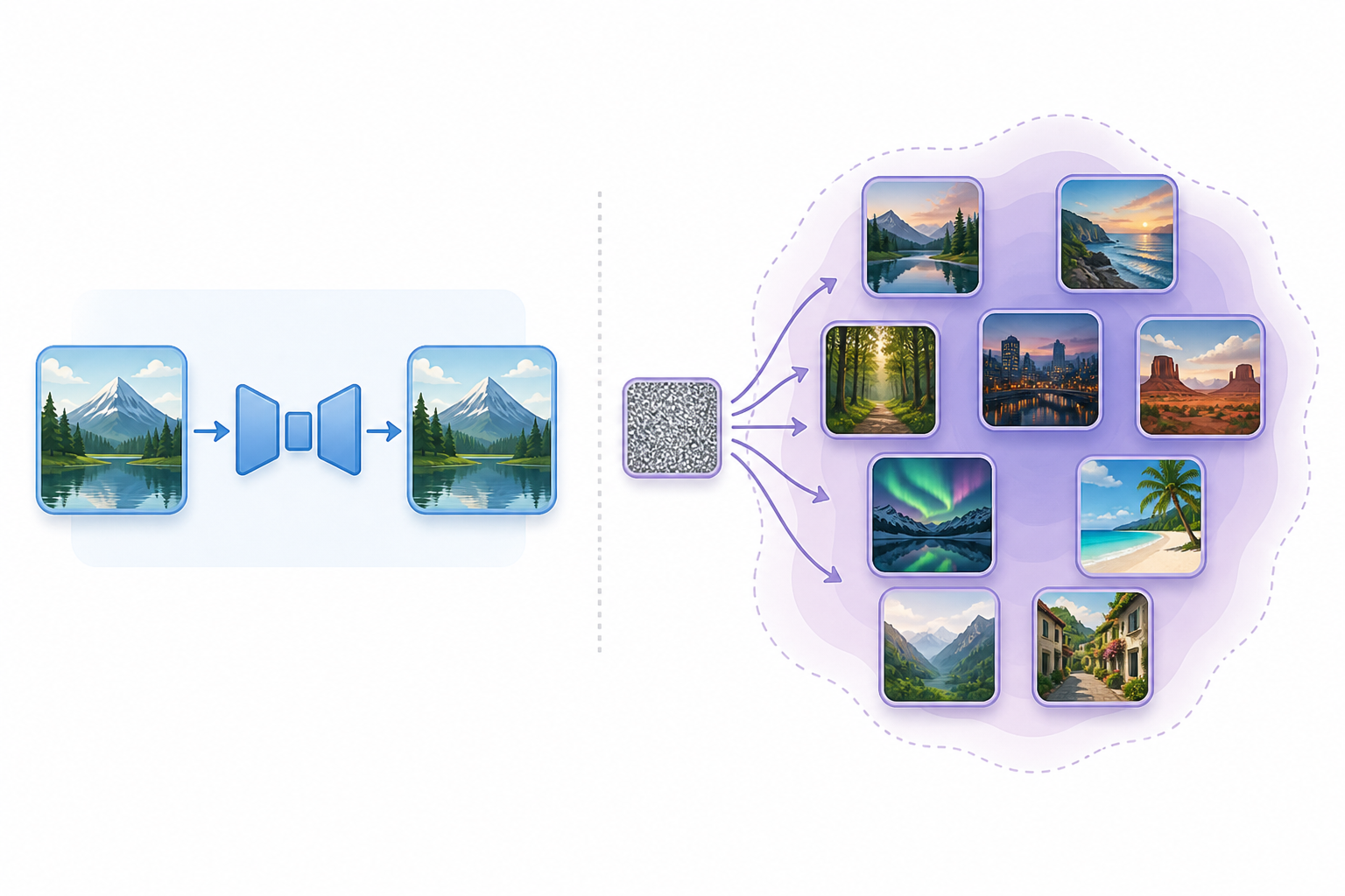
The difficulty of evaluating the quality of generative models fundamentally stems from the fact that generation tasks do not have a single correct answer. For image reconstruction, the output can be directly compared with a ground-truth image, making pointwise metrics such as PSNR and SSIM reasonable choices.² In contrast, for image generation, there may be many plausible outputs under the same condition. Therefore, the evaluation objective is no longer to determine whether a single sample matches a standard answer, but rather to assess whether the generated distribution is close to the real data distribution.

Likelihood evaluation

Log-likelihood is a tempting evaluation criterion because a generative model is supposed to assign high probability to realistic data. For conditional generation, the analogous quantity is

where $x$ is an image and $c$ is the text prompt. If likelihood were a good prompt-alignment metric, images with higher likelihood under a prompt should also receive higher CLIP scores for that prompt.

A simple SD3.5-Large experiment tests this directly. For each prompt, multiple images are generated, each image is scored by latent likelihood $\log p_\theta(x \mid c)$, and the same image is scored by CLIP. The relevant statistic is the within-prompt Spearman correlation between likelihood and CLIP score, because raw pooling across prompts is confounded by prompt-specific likelihood offsets.

The correlations are small. Even in the statistically positive setting, the effect size is weak. This means CLIP score and likelihood are measuring different things: CLIP measures text-image alignment in a learned representation space, while likelihood measures density under the model’s latent distribution. Higher likelihood does not reliably imply better CLIP alignment.

Therefore, likelihood is useful as a density diagnostic, but it should not be treated as an automatic evaluation metric for prompt following or perceptual quality.

On the other hand, although human evaluation is closest to the ultimate objective, large-scale, reproducible, and statistically reliable human studies are costly and difficult to use as a routine evaluation protocol. Therefore, designing automatic, reproducible evaluation metrics that align well with human perception has become one of the central problems in generative model research.

2. Discriminative models as a natural thought

The natural escape from pixel space is representation space. Directly comparing generated and real images in pixel space is usually not meaningful: a small translation, crop, lighting change, or texture variation can produce a large pixel difference, even when two images look similar to humans. More importantly, the goal of generative model evaluation is not to check whether one generated image exactly matches one reference image, but to ask whether the model produces samples that are realistic, diverse, and semantically close to the real data distribution.

A pretrained discriminative model gives us a practical proxy for this question. Instead of comparing images as raw arrays, we pass them through a feature extractor and compare their embeddings. If the feature extractor has learned useful visual concepts, then nearby points in feature space should share higher-level properties such as object category, shape, texture, composition, or image-text alignment. In this view, the feature extractor becomes the measuring instrument: it decides which differences are important and which differences can be ignored.

Once images are represented as features, several evaluation strategies become possible. We can ask whether each generated image is confidently recognized by a classifier, which leads to Inception Score.³ We can ask whether generated samples lie close to the real data manifold and whether they cover it, which leads to precision and recall.⁴ Later, we can compare the full real and generated feature distributions, which leads to FID.⁷

This idea appears in many forms:

• use an ImageNet classifier to judge whether generated images look like recognizable objects.³
• use its intermediate features to compare real and generated distributions.⁷
• use CLIP-like features to evaluate image-text alignment.¹⁶
• use self-supervised features such as DINO for more general visual similarity.¹⁰
• use video encoders for temporal and motion-aware evaluation.¹⁷

The representation model becomes a measuring device. It is not the generator, but it defines what the evaluation can see.

2.1 Inception Score

Inception Score³ was one of the early popular representation-based metrics for image generation. It uses a pretrained Inception classifier and rewards two things:

1. each generated image should produce a confident class prediction;
2. the full generated set should cover many classes.

Written roughly, it is

The intuition is attractive. If each image is sharp and recognizable, $p(y \mid x)$ should have low entropy. If the generator is diverse, the marginal class distribution $p(y)$ should have high entropy. So the score tries to reward both fidelity and diversity.

But Inception Score also shows the danger of representation-based evaluation. It does not compare to the real data distribution directly. It mostly cares about classifier-recognizable ImageNet categories. It can reward samples that are easy for the classifier while missing other aspects of realism. It also has little to say about conditional generation unless the condition is aligned with the classifier labels.

Still, it introduced an important pattern: use a strong pretrained model as a proxy for human visual judgment.

2.2 Precision and recall

Precision and recall for generative models⁴ take the real data distribution into consideration.

• Precision asks whether generated samples lie near the real data manifold.
• Recall asks whether the generated distribution covers the real data manifold.

The original precision-recall-distribution method starts by embedding real and generated samples into a feature space, usually with a pretrained classifier. It then clusters the pooled embeddings into bins and estimates two discrete distributions: $p_b$ for real data and $q_b$ for generated data. By sweeping a slope parameter $\lambda$, it obtains a precision-recall curve:

This curve is useful, but it depends on density estimates after clustering. The improved precision and recall metric⁵ instead builds explicit non-parametric approximations of the real and generated manifolds in feature space. Let $R=\lbrace r_i \rbrace$ be real features and $G=\lbrace g_j \rbrace$ be generated features. For each real feature $r_i$, let $\rho_i$ be the distance from $r_i$ to its $k$th nearest neighbor among real features, and define the real manifold estimate as

The generated manifold estimate $\mathcal{M}_G$ is defined the same way using generated features and their $k$th-neighbor radii. Precision and recall are then simple membership tests:

So high precision means most generated samples fall inside the real-data manifold estimate. High recall means the generated manifold covers most real-data samples. The important point is that the two numbers separate sample realism from distribution coverage instead of forcing both questions into one scalar.

3. One score that rules them all

Then came FID, which was introduced in the TTUR paper⁷ and has since become a default metric for generative model evaluation.

3.1 What is FID?

Frechet Inception Distance compares real and generated samples in Inception feature space. Instead of asking whether individual samples are classified confidently, it fits a Gaussian to the real features and another Gaussian to the generated features:

Here $(\mu_r, \Sigma_r)$ are the mean and covariance of real features, and $(\mu_g, \Sigma_g)$ are the mean and covariance of generated features. Lower is better. Three characteristics of FID are worth keeping in mind:

1. Finite-sample estimate. FID is not computed from the full model distribution. In practice, people usually generate 50k samples and use their features to represent the generated distribution. This makes FID easy to standardize, but it also means the score can depend on sample count, random seed, and which finite sample set happens to be evaluated.
2. Gaussian assumption. FID reduces each feature distribution to a mean and covariance, then computes the distance between the two fitted Gaussians. This makes the metric simple and stable to report, but it also means that any structure beyond second-order statistics is invisible to the score.
3. Fréchet Distance. After the Gaussian approximation, FID uses the Fréchet distance between the two Gaussian distributions, also known as the 2-Wasserstein distance in this setting. The mean term measures how far the centers of the real and generated feature clouds are from each other, while the covariance term measures how different their spreads and correlations are.

3.2 Variants of FID

FD_∞⁸ challenges the finite-sample behavior of FID. In practice, FID is computed from a finite number of real and generated samples, so the estimated means and covariances introduce bias. The idea of FD_∞ is to view the reported score as a finite-sample estimate $\mathrm{FD}_N$ and extrapolate toward the value that would be obtained with infinitely many samples:

The conclusion is stronger than “FID needs enough samples.” Finite-sample FID is biased, and the bias depends on the model being evaluated. Therefore, fixing the protocol at 50k samples does not fully remove the issue: one model may look better partly because its finite-sample bias is smaller. FD_∞ improves the estimator, but it does not change the underlying assumptions of FID: Gaussian feature distributions and a fixed representation space.

Kernel Inception Distance, or KID⁹, challenges the Gaussian assumption behind FID. It keeps the same broad idea of comparing real and generated samples in Inception feature space, but replaces the Gaussian Fréchet distance with a kernel maximum mean discrepancy (MMD). If $u=\phi(x)$ is a real feature and $v=\phi(\tilde{x})$ is a generated feature, then the squared MMD is

KID usually uses a polynomial kernel on Inception features:

where $d$ is the feature dimension. Given real features $\lbrace u_i \rbrace_{i=1}^m$ and generated features $\lbrace v_j \rbrace_{j=1}^n$, an unbiased finite-sample estimator is

This unbiased estimator is one reason KID is useful when the number of evaluation samples is limited, while FID can be biased for finite sample sizes.

FD-DINO¹⁰ challenges a different part of FID: the feature extractor. Standard FID computes Fréchet distance in Inception feature space, so the metric inherits the priorities and blind spots of a supervised ImageNet classifier. FD-DINO keeps the same Fréchet-distance calculation, but replaces Inception features with DINO or DINOv2 representations.

The motivation is that self-supervised visual features can capture semantic similarity without being as tightly tied to ImageNet classification labels. In this view, the distance formula is not the only thing that matters; the representation space defines what the metric can see. If DINO places semantically similar images closer together, then a Fréchet distance in DINO feature space may better reflect perceptual similarity for modern generators, especially diffusion models.

FD-DINO is therefore less a new distance than a reminder that evaluation metrics are pipelines. Changing the encoder can change the meaning of the same mathematical score.

3.3 Extending FID beyond image generation

The same idea has been used far beyond unconditional image generation. In text-to-image evaluation, MS COCO¹⁸ became a common reference point because it contains natural images paired with human-written captions. The common zero-shot setting is usually called FID-30K on COCO: sample 30,000 captions from the MS COCO 2014 validation split, generate one image for each caption, and compare those 30,000 generated images against the reference images from the full COCO validation set, which contains 40,504 images.¹⁹ This makes the result easy to compare across papers, but it is still a distribution-level image metric: a model can improve COCO FID without necessarily improving prompt faithfulness for every individual caption.

For video, the analogous metric is often FVD, Fréchet Video Distance¹⁷. There is no single COCO-like prompt set for FVD, because the reference set depends on the video task: video prediction, unconditional video generation, text-to-video generation, or domain-specific generation may all use different datasets. In the original FVD paper, the authors evaluate on datasets such as BAIR robot pushing, KTH actions, and their StarCraft 2 Videos benchmark. They use I3D video features, especially the logits of an I3D model trained on Kinetics-400, and report FVD with 256 validation samples for BAIR and 1024 samples for KTH and SCV. Many later video-generation papers use 2048 real and generated clips, so the number of clips, clip length, resolution, and feature backbone should always be reported together with the score.

Instead of embedding single images with Inception, FVD embeds short video clips with a video understanding network, then computes the same Gaussian Fréchet distance in that video feature space:

Here the means and covariances are computed from video features rather than image features. This matters because video generation is not only about whether each frame looks realistic. The model also has to maintain identity, geometry, motion, and temporal coherence across frames, so a frame-level FID can miss failures such as flicker, frozen motion, or inconsistent object dynamics.

4. The problem with FID

FID is useful, but it is not perfect. For a long time, FID dominated generative model evaluation: train a model, generate samples, compute FID, and use the number to compare methods. As generative models become more powerful, the problems of FID have become harder to ignore: the score is useful, influential, and still only a proxy.

4.1 How stable is FID?

The first problem is stability. FID can move for reasons that have little to do with the conceptual quality of the generator.

4.1.1 Randomness in training

Random seeds, data order, initialization, augmentation randomness, and hardware-level nondeterminism can all change the final model. If the reported improvement is small, it may be hard to know whether the method improved the generator or simply landed on a better run.

The FID Lottery makes this problem explicit.¹³ The paper treats FID as a random variable over two axes: the training seed used to obtain the model and the generation seed used to draw the evaluation samples. On class-conditional ImageNet 256x256, it finds that retraining the same recipe with a different seed moves FID much more than simply resampling from a fixed network. The spread comes from ordinary sources of training randomness, including initialization, data order, and per-step Gaussian noise in the flow-matching loss. The conclusion is practical: a single FID number from one model checkpoint is a lottery ticket. Small gaps should be treated as inconclusive unless they are larger than the measured variation, and strong claims should report error bars over multiple training seeds.

The between-seed standard deviation is about three times larger than the within-seed sampling noise, so evaluating more samples from one checkpoint cannot remove the dominant uncertainty. The model itself has to be retrained under multiple seeds.

4.1.2 Differences in evaluation pipeline

FID is also sensitive to image processing details:

• the exact feature extractor;
• image resolution and preprocessing;
• resizing and cropping implementation;
• color space and normalization;
• image format and compression;
• choice of reference set.

This matters because a reported FID is not just a property of the model. It is a property of the whole evaluation pipeline.

Parmar, Zhang, and Zhu make this point concrete in On Aliased Resizing and Surprising Subtleties in GAN Evaluation.¹² Their paper shows that low-level preprocessing choices such as resizing and compression can create surprisingly large FID changes. The key issue is aliasing: when images are downsampled, the prefilter should change with the downsampling factor, but common bilinear and bicubic resizing implementations often use a fixed-width filter. That can introduce aliasing artifacts, which then corrupt the Inception features used by FID. They also show that JPEG compression can affect the downstream score; if the real training images are compressed, compressing the generated images can even improve FID without making the generator better. The lesson is simple: FID is not only measuring the generator. It is also measuring the hidden image-processing pipeline around the generator.

The reference set is another hidden source of variation. FID compares generated samples to a chosen set of real-image features, so changing that real set changes the target distribution. This is not just a constant offset. In one ImageNet-256 check, the exact same generated samples were scored against three reference sets: 50k validation images, a random 50k subset of training images, and a larger training-set reference. Moving from the validation reference to a training-set reference changed different models in different directions: for one model, FID improved because its samples were closer to the training distribution; for another, FID worsened because its samples happened to sit closer to the validation distribution.

This example separates two effects. First, reference size matters: going from 50k training images to a much larger training reference lowered FID consistently. Second, reference distribution matters: validation images and training images are not the same target, and the shift is model-dependent. The consequence can be severe enough to flip rankings. In the table above, VA-VAE looks slightly better than RAE against the validation reference, but RAE looks better against the training-based references. Therefore, a paper should not only report “FID”; it should say exactly which reference statistics were used.

4.2 When FID score becomes unsuggestive

The second problem is meaning. Today, many ImageNet generation papers compete over very small FID gaps, sometimes smaller than 0.2. At that scale, the number can look precise while saying very little about what changed perceptually: did the model become more diverse, more faithful, more useful, or simply better aligned with the evaluation pipeline?

4.2.1 Do FID gains on ImageNet transfer?

FID is a feature-space metric. If the feature extractor cannot see a failure, FID may not punish it. Inception features are good for many natural-image semantics, but they are not a universal model of human perception. They may underweight counting, spatial relations, text rendering, fine-grained attributes, unusual styles, or domain-specific details.

DiffusionBench makes this transfer problem concrete.¹⁴ The paper argues that DiT research has become overly centered on class-conditional ImageNet, where methods are often compared by FID and nearby distribution metrics. To test whether that progress transfers, it introduces NanoGen, a unified training and evaluation framework that can train comparable ImageNet and text-to-image DiT models with only a small configuration change. After training 21 latent diffusion models across VAE, RAE, pixel-space, and MeanFlow-style settings, the paper finds no strong positive relationship between ImageNet performance and text-to-image performance. In fact, the reported Pearson correlations between ImageNet and T2I rankings are negative, between -0.377 and -0.580 across three metrics.

The conclusion is not that ImageNet FID is useless. It is that ImageNet FID is local evidence. A method can improve class-conditional ImageNet generation without improving prompt-following, compositionality, or the behavior users actually care about in text-to-image systems. If the claim is broad progress in generative modeling, ImageNet FID alone is too narrow a witness.

4.2.2 Small FID absolute value loss its meaning

The FID Lottery already shows one reason small gaps are dangerous: retraining the same recipe with different random seeds can move FID more than the improvement claimed by many papers.¹³ Even before asking whether the metric reflects human preference, we have to ask whether the reported gap is larger than the noise induced by training randomness, sampling randomness, and evaluation details.

Even if the model and reference distribution are fixed, a finite 50k reference has its own sampling variance. In 100 independent random 50k draws from ImageNet training images, the estimated FID floor varied as follows:

The variance is small, but not zero. Around model FIDs of 3 to 5, this corresponds to fluctuations on the order of a few hundredths. Combined with the FID Lottery result, this makes tiny FID gaps hard to interpret. A difference of 0.05, 0.1, or even 0.2 may reflect the seed, the reference set, preprocessing, or sample count more than a meaningful change in generative behavior. In this regime, a small FID gap cannot suggest much by itself.

4.2.3 FID score on other domains is even worse

The problem becomes sharper once generation becomes conditional. Text-to-image is the simplest example. In class-conditional ImageNet generation, the condition is a single label, and FID can at least ask whether the generated image distribution looks like the ImageNet distribution. In text-to-image, the condition is open-ended language. The model has to follow arbitrary prompts faithfully and produce visually convincing images at the same time. MiniT2I makes this distinction explicit: it reports MSCOCO-30K FID as a distribution-level realism metric, but notes that this metric does not ask whether the generated image actually followed the prompt.³⁶

This is exactly where FID becomes weak. A generated image can be sharp, natural, and close to the COCO image distribution while still missing the requested object, count, spatial relation, text, style, or rare concept. Conversely, an image can follow a strange prompt faithfully while looking less typical under an Inception feature distribution. For T2I, the central question is not only “does this look like a real image?” It is also “does this image satisfy this sentence?” FID only sees the first question.

5. Benchmarks become the new standard

This is why text-to-image evaluation quickly moves beyond FID toward prompt-following benchmarks, VQA-based checks, OCR, image-text alignment, and human preference. FID can still be useful as a realism signal, but for T2I it is no longer enough to describe the model’s behavior.

5.1 What benchmarks do

Instead of asking only whether generated samples match a broad reference distribution, benchmarks ask whether models solve curated tasks. In practice, a benchmark usually contains a prompt suite, a generation protocol, and an automatic evaluator. The evaluator is often another pretrained model: an object detector, segmentation model, VQA model, captioning model, CLIP-like encoder, video encoder, optical-flow estimator, or MLLM judge. So the score is not an abstract measurement of “quality”; it is a task-specific measurement of whether the generated output satisfies what the benchmark and its verifier know how to check.

The table below is not exhaustive, but it shows how the evaluator changes with the task.

This is progress. Benchmarks make failure modes visible. They turn vague complaints into testable categories. They also help evaluation move closer to actual use cases.

But benchmarks are not perfect. GenEval is a useful example: it made text-to-image failures concrete by checking object presence, count, position, color, and attribute binding with a fixed detector-and-classifier pipeline, but that also means it can be easy to hack. For example, a model trained on BLIP-3o data can reach a GenEval score of 0.67, surpassing SD3.5-M with a GenEval score of 0.63. A higher GenEval score can therefore mean better prompt following, but it can also mean better adaptation to GenEval itself.

5.2 Pass@k reveals distribution coverage

Benchmark scores usually ask whether one generated output follows the prompt, satisfies a verifier, or passes a task-specific check. In that sense, they are often alignment metrics: they tell us whether a sample matches what the prompt or benchmark asks for.

Pass@k pushes this idea closer to distribution-level evaluation by asking how the score changes as we draw more samples from the same model. A single benchmark score mainly measures the success probability of a typical draw; pass@k asks whether the model’s conditional distribution contains many different successful outputs, or whether probability mass has concentrated on a narrow set of evaluator-favored samples.³²

For each prompt, generate $n$ independent samples and let $c$ be the number that pass the benchmark verifier. The pass@k estimator asks whether at least one sample in a size-$k$ subset succeeds:

Pass@1 recovers the ordinary single-sample benchmark score under the same evaluator. Larger $k$ asks a different question: if we sample more from the same model, does the distribution contain more successful generations for the prompt? If a method improves pass@1 but the pass@k curve saturates early, the method may be improving one-shot sampling efficiency or prompt-following alignment while reducing distribution coverage. If the curve keeps rising at larger $k$, it suggests that the model assigns probability to a broader set of successful outputs.

6. Closing thought

So we end up with a layered evaluation stack:

The history of generative model evaluation is a history of proxies. Pixels were too brittle, so we moved to representations. Inception Score was too indirect, so we moved to FID. FID was too coarse, so we built variants with better features and video encoders. Distribution metrics missed conditional behavior, so we built benchmarks. Benchmarks became targets, so we added human evaluation and failure audits.

Each step fixes something and exposes something else.

None of these metrics is perfect. A useful evaluation should therefore look at a model from multiple angles: distribution distance, precision and recall, benchmark scores, pass@k behavior, and qualitative failures.

As the old saying goes, beauty is in the eye of the beholders. No automatic metric can truly replace human evaluation. Evaluating generative models still has a long way to go. Metrics can make evaluation cheaper, faster, and more reproducible, but the final question is still whether people find the generated output good, faithful, useful, or meaningful.

@misc{wang2026struggling,
  title = {Struggling Toward Generative Model Evaluation},
  author = {Wang, Yifei},
  year = {2026},
  url = {https://a-little-hoof.github.io/blog/how-to-evaluate-your-generative-model/},
  note = {Blog post}
}

References

- Song, Sohl-Dickstein, Kingma, Kumar, Ermon, & Poole. Score-Based Generative Modeling through Stochastic Differential Equations. ICLR 2021. arXiv:2011.13456.
- Wang, Bovik, Sheikh, & Simoncelli. Image quality assessment: from error visibility to structural similarity. IEEE Transactions on Image Processing, 13(4):600-612, 2004. doi:10.1109/TIP.2003.819861.
- Salimans, Goodfellow, Zaremba, Cheung, Radford, & Chen. Improved Techniques for Training GANs. NeurIPS 2016. arXiv:1606.03498.
- Sajjadi, Bachem, Lucic, Bousquet, & Gelly. Assessing Generative Models via Precision and Recall. NeurIPS 2018. arXiv:1806.00035.
- Kynkäänniemi, Karras, Laine, Lehtinen, & Aila. Improved Precision and Recall Metric for Assessing Generative Models. NeurIPS 2019. arXiv:1904.06991.
- Gretton. ICLR 2026 course PDF. PDF.
- Heusel, Ramsauer, Unterthiner, Nessler, & Hochreiter. GANs Trained by a Two Time-Scale Update Rule Converge to a Local Nash Equilibrium. NeurIPS 2017. arXiv:1706.08500.
- Chong & Forsyth. Effectively Unbiased FID and Inception Score and where to find them. CVPR 2020. arXiv:1911.07023.
- Bińkowski, Sutherland, Arbel, & Gretton. Demystifying MMD GANs. ICLR 2018. arXiv:1801.01401.
- Stein, Cresswell, Hosseinzadeh, Sui, Ross, Villecroze, Liu, Caterini, Taylor, & Loaiza-Ganem. Exposing flaws of generative model evaluation metrics and their unfair treatment of diffusion models. NeurIPS 2023. arXiv:2306.04675.
- Lucic, Kurach, Michalski, Gelly, & Bousquet. Are GANs Created Equal? A Large-Scale Study. NeurIPS 2018. arXiv:1711.10337.
- Parmar, Zhang, & Zhu. On Aliased Resizing and Surprising Subtleties in GAN Evaluation. CVPR 2022. arXiv:2104.11222.
- Yang, Geng, Ju, Tian, & Wang. Representation Fréchet Loss for Visual Generation. arXiv 2026. arXiv:2604.28190.
- Dufour, Efros, & Pérez. The FID Lottery: Quantifying Hidden Randomness in Generative-Model Evaluation. arXiv 2026. arXiv:2606.20536.
- Leng, Singh, Liang, Smith, Bell, Saha, Yuan, & Zheng. DiffusionBench: On Holistic Evaluation of Diffusion Transformers. arXiv 2026. arXiv:2606.24888.
- Radford, Kim, Hallacy, Ramesh, Goh, Agarwal, Sastry, Askell, Mishkin, Clark, Krueger, & Sutskever. Learning Transferable Visual Models From Natural Language Supervision. ICML 2021. arXiv:2103.00020.
- Unterthiner, van Steenkiste, Kurach, Marinier, Michalski, & Gelly. Towards Accurate Generative Models of Video: A New Metric & Challenges. arXiv 2018. arXiv:1812.01717.
- Lin, Maire, Belongie, Bourdev, Girshick, Hays, Perona, Ramanan, Zitnick, & Dollár. Microsoft COCO: Common Objects in Context. ECCV 2014. arXiv:1405.0312.
- Saharia, Chan, Saxena, Li, Whang, Denton, Ghasemipour, Gontijo Lopes, Karagol Ayan, Salimans, Ho, Fleet, & Norouzi. Photorealistic Text-to-Image Diffusion Models with Deep Language Understanding. NeurIPS 2022. NeurIPS paper.
- Ghosh, Hajishirzi, & Schmidt. GenEval: An Object-Focused Framework for Evaluating Text-to-Image Alignment. NeurIPS 2023. arXiv:2310.11513.
- Hu, Wang, Fang, Fu, Cheng, & Yu. ELLA: Equip Diffusion Models with LLM for Enhanced Semantic Alignment. ECCV 2024. arXiv:2403.05135.
- Kamath, Chang, Krishna, Zettlemoyer, Hu, & Ghazvininejad. GenEval 2: Addressing Benchmark Drift in Text-to-Image Evaluation. arXiv 2025. arXiv:2512.16853.
- Li, Lin, Pathak, Li, Fei, Wu, Ling, Xia, Zhang, Neubig, & Ramanan. GenAI-Bench: Evaluating and Improving Compositional Text-to-Visual Generation. CVPR Workshops 2024. arXiv:2406.13743.
- Huang, Sun, Xie, Li, & Liu. T2I-CompBench: A Comprehensive Benchmark for Open-world Compositional Text-to-image Generation. NeurIPS 2023. arXiv:2307.06350.
- Huang, He, Yu, Zhang, Si, Jiang, Zhang, Wu, Jin, Chanpaisit, Wang, Chen, Wang, Lin, Qiao, & Liu. VBench: Comprehensive Benchmark Suite for Video Generative Models. CVPR 2024. arXiv:2311.17982.
- Sun, Huang, Liu, Wu, Xu, Li, & Liu. T2V-CompBench: A Comprehensive Benchmark for Compositional Text-to-video Generation. CVPR 2025. arXiv:2407.14505.
- Ma, Ji, Ye, Lin, Wang, Zheng, Zhou, Sun, & Ji. I2EBench: A Comprehensive Benchmark for Instruction-based Image Editing. NeurIPS 2024. arXiv:2408.14180.
- Qian, Lu, Fu, Wang, Chen, Yang, Hu, & Gan. GIE-Bench: Towards Grounded Evaluation for Text-Guided Image Editing. arXiv 2025. arXiv:2505.11493.
- He, Bai, Lin, Zhao, Hu, Sheng, Yi, Li, & Liu. T3Bench: Benchmarking Current Progress in Text-to-3D Generation. arXiv 2023. arXiv:2310.02977.
- Zhang, Zhang, Wu, Wang, Wetzstein, Lin, & Liu. 3DGen-Bench: Comprehensive Benchmark Suite for 3D Generative Models. arXiv 2025. arXiv:2503.21745.
- Yue et al. MMMU: A Massive Multi-discipline Multimodal Understanding and Reasoning Benchmark for Expert AGI. CVPR 2024. arXiv:2311.16502.
- Wang, Wu, Fu, Chen, Chen, Gan, & Wei. Sharper, Not Broader: Pass@k Reveals Mode Collapse in Guided and Distilled Diffusion. Draft manuscript, 2026.
- Zheng, Ma, Tong, & Xie. Diffusion Transformers with Representation Autoencoders. arXiv 2025. arXiv:2510.11690.
- Yue, Hu, Chen, Zhang, Pan, Liu, Wang, Lan, Zhu, Zheng, & Wang. What Matters for Diffusion-Friendly Latent Manifold? Prior-Aligned Autoencoders for Latent Diffusion. arXiv 2026. arXiv:2605.07915.
- Yao & Wang. Reconstruction vs. Generation: Taming Optimization Dilemma in Latent Diffusion Models. arXiv 2025. arXiv:2501.01423.
- Wang et al. A Minimalist Baseline for Text-to-Image Generation. Blog post, 2026. https://peppaking8.github.io/#/post/minit2i.
Please Cite
If this post is useful for your work, please cite it as: